STUDIO 02.2: GEE TUTORIAL
Premise and Objectives
This tutorial requires NO coding experience or familiarity with GEE. You MUST have an approved account to use GEE: https://earthengine.google.com/signup.
This tutorial will serve to act as a showcase of some capabilities that are possible with GEE. It is NOT meant to cover every detail of coding in GEE. We will cover a few basics of GEE using javascript (see note at the end about using python):
1. Overview
2. Datasets
3. Graphical User Interface (GUI)
4. Climate Projection - Rasters
5. Features - Shapes
6. Importing data into GEE
7. Exporting data out of GEE
8. Further resources
The workflow will specifically involve running a simple climate projection analysis using temperature over an imported shape area and exporting the results in a format we can use in GIS. If you ever get lost or run into errors, a clean working version of the code is posted at the end.
Overview
What is GEE? GEE is the most advanced cloud-based geospatial processing platform in the world. It combines a multi-petabyte catalog of satellite imagery and geospatial datasets with planetary-scale analysis capabilities and makes it available for scientists, researchers, and developers to detect changes, map trends, and quantify differences on the Earth's surface. https://earthengine.google.com/

Combining science with massive data and technology resources in this way offers these advantages:
• Unprecedented speed: On a top-of-the-line desktop computer, it can take days or weeks to compute an analysis over any large portion of the earth. Using our cloud-based computing power, we can reduce that by orders of magnitude.
• Ease of use and lower costs: An online platform that offers easy access to data, scientific algorithms, and computation power from any web browser can dramatically lower the cost and complexity for analysis of geospatial data.
Datasets
GEE has complete archives of Landsat 4,5,7, and 8 that have been processed by the United States Geological Survey (USGS), a wide variety of Moderate Resolution Imaging Spectro-Radiometer (MODIS) data products as global composites, and many other remotely-sensed and ancillary image data products. In recent years, GEE has been processing huge amounts of demographic data along with climate and weather data including outputs from climate models. All data are pre-processed, georeferenced, and ready for use. Users may also upload their own raster and vector data, which can be kept private or made publicly available. https://developers.google.com/earth-engine/datasets
In GEE, a single raster is an image while a collection of rasters is known as an image collection. Shapes are known as features and feature collections.
Graphical User Interface (GUI)
Access here: https://code.earthengine.google.com/
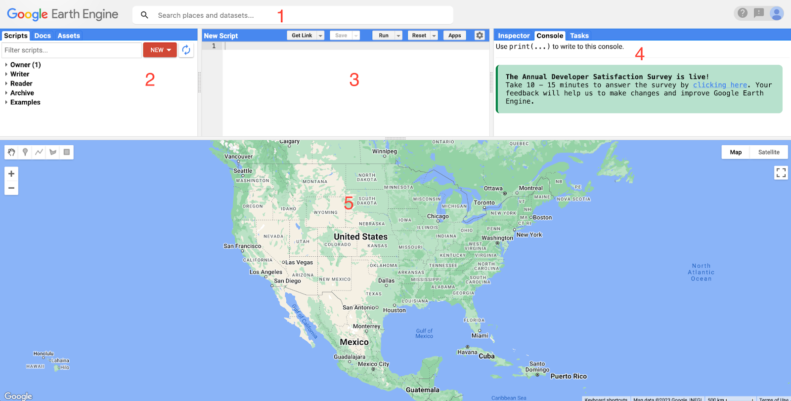 1. Search bar: find places, data sets, tables, etc
2. Access scripts, documentation on all GEE functions, and assets
3. Scripting window
4. Inspector, Console, Tasks
5. Map
Climate Projection - Rasters
We will begin by searching for climate model projections that are pre-processed in GEE. In the search bar, type
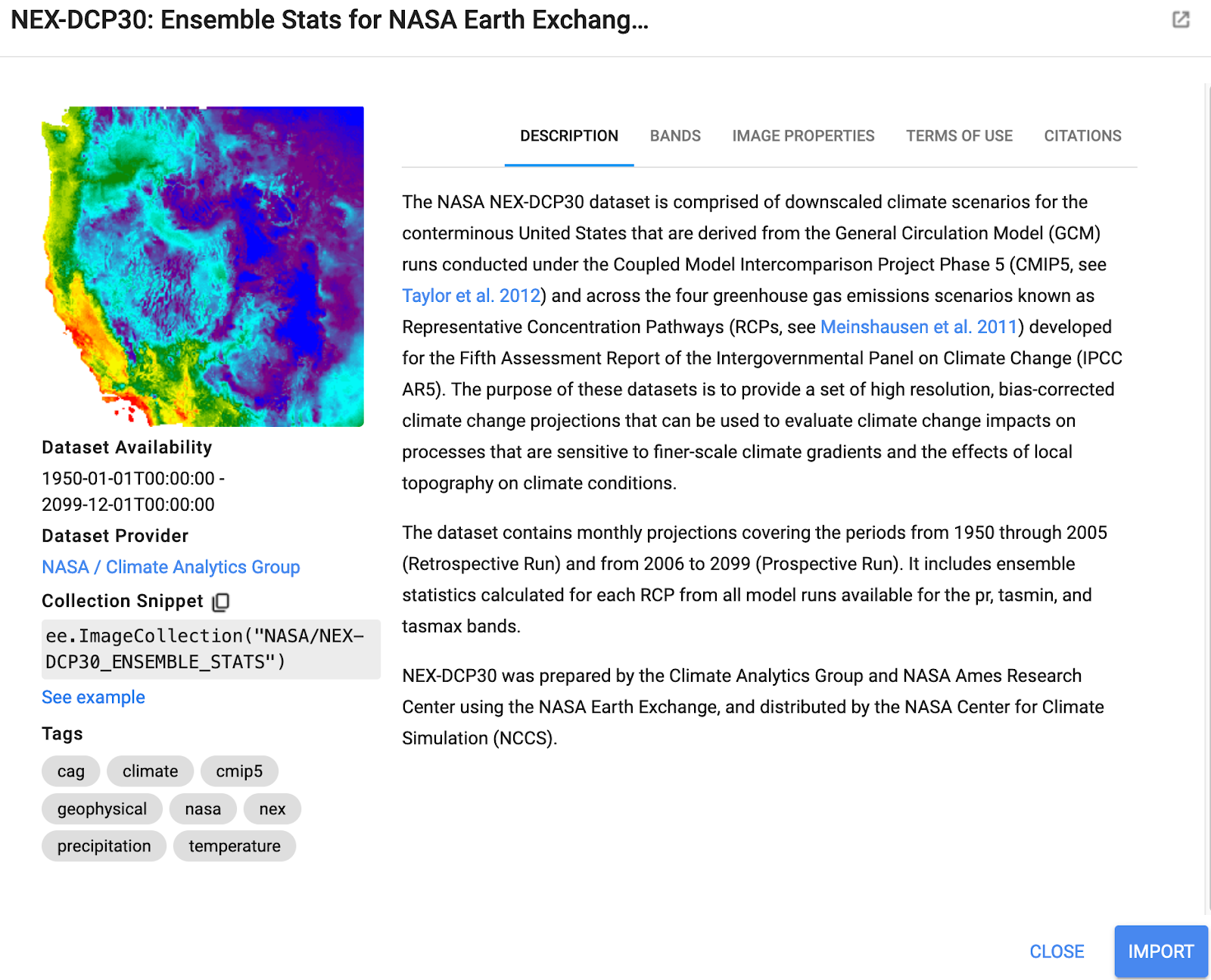
A panel with information on the dataset should pop up. This dataset is based on the Coupled Model Intercomparison Project Phase 5 or CMIP5. This is a collection of climate models each run by different institutions (over 30!) such as: NASA (National Aeronautics and Space Administration), the Norwegian Climate Centre, and the Japan Agency for Marine-Earth Science and Technology. The dataset conveniently provides us with “ensemble” stats - in this case a “multi-model ensemble” - meaning it takes the average of all the models in CMIP5. As an aside, if we wanted to work with CMIP5 data directly and calculate an ensemble mean, we would have to download and process terabytes of data. The data is “down-scaled” which means that it has been converted to a higher resolution (smaller pixels) using various methods that incorporate observations (see citations in the dataset panel for more info) and the data only covers the U.S..
The data is monthly and spans from 1950-2099 with historical (1950-2005) and projected (2006-2099) runs. The projections are further split into three categories based on Representative Concentration Pathways or RCPs - RCP2.6, RCP4.5, and RCP8.5. These pathways represent different levels of greenhouse gas concentrations with the number next to “RCP” indicating the radiative forcing in W/m^2 (higher number = warmer climate). There are various variables we can work with such as precipitation or near surface temperature (see the
In the code editor, type:
This line declares the variable

You should run into this error on your console (right panel). To preserve computation on GEE’s servers, GEE limits the query to 5000 elements. Instead of trying to grab the entire dataset, let’s just inspect the first image using the
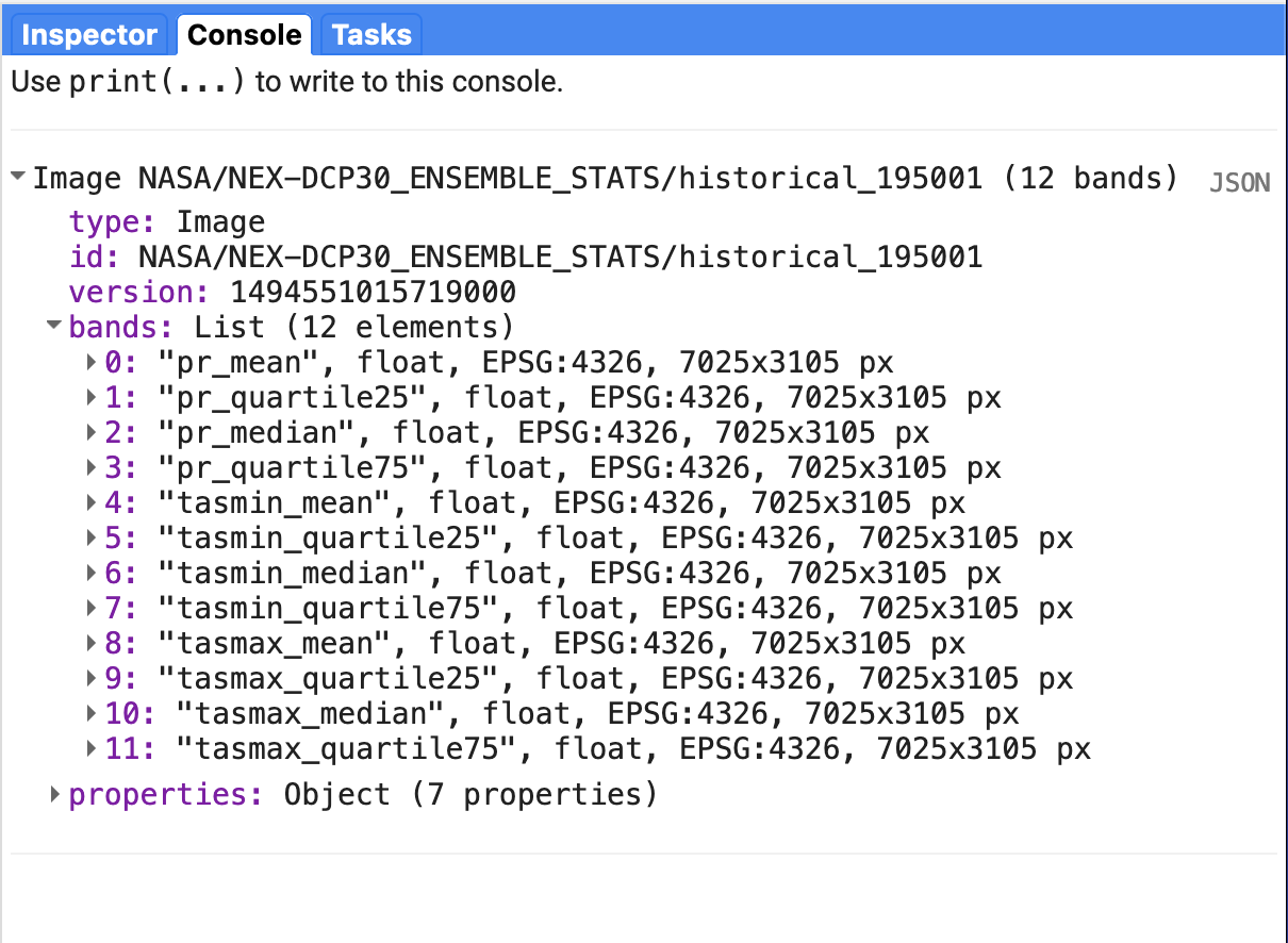
If we go to the console tab, we should see our sample image with further information. Be sure to always do a check of your data in this way before trying any analysis so that you understand the organization of the data.
For a climate change analysis, we need a historical and a projected dataset to compare. We will use the first 3 decades from the historical runs (1950-1979) and last 3 decades from the projected runs (2070-2099) and examine how minimum surface temperatures during the summer have changed across the century. Climate analyses try to work with at least 3 decades of data to remove noise from natural year-to-year variability. Minimum temperatures can be thought of as nighttime temperatures while maximum temperatures can be thought of as the daytime temperatures. Under climate change, nighttime temperatures are increasing at a faster rate than daytime temperatures for most regions. During summer months, we rely on cool nighttime temperatures to recover from heat stress so being able to project the future trends is crucial with regards to human health. Let’s extract just what we need from the entire dataset as described above.
The “//” indicates that the text that follows it is not meant to be evaluated but rather used as comments. Without getting into the weeds of each method, the code:
> first brings in the entire NEX-DCP30 ensemble image collection
> selects only the images in the collection that correspond to the band or variable we are interested in (
> filters the images further for only the
> filters further for the first 3 decades
> filters further for the summer months
> finally take the mean of all the remaining images
If we
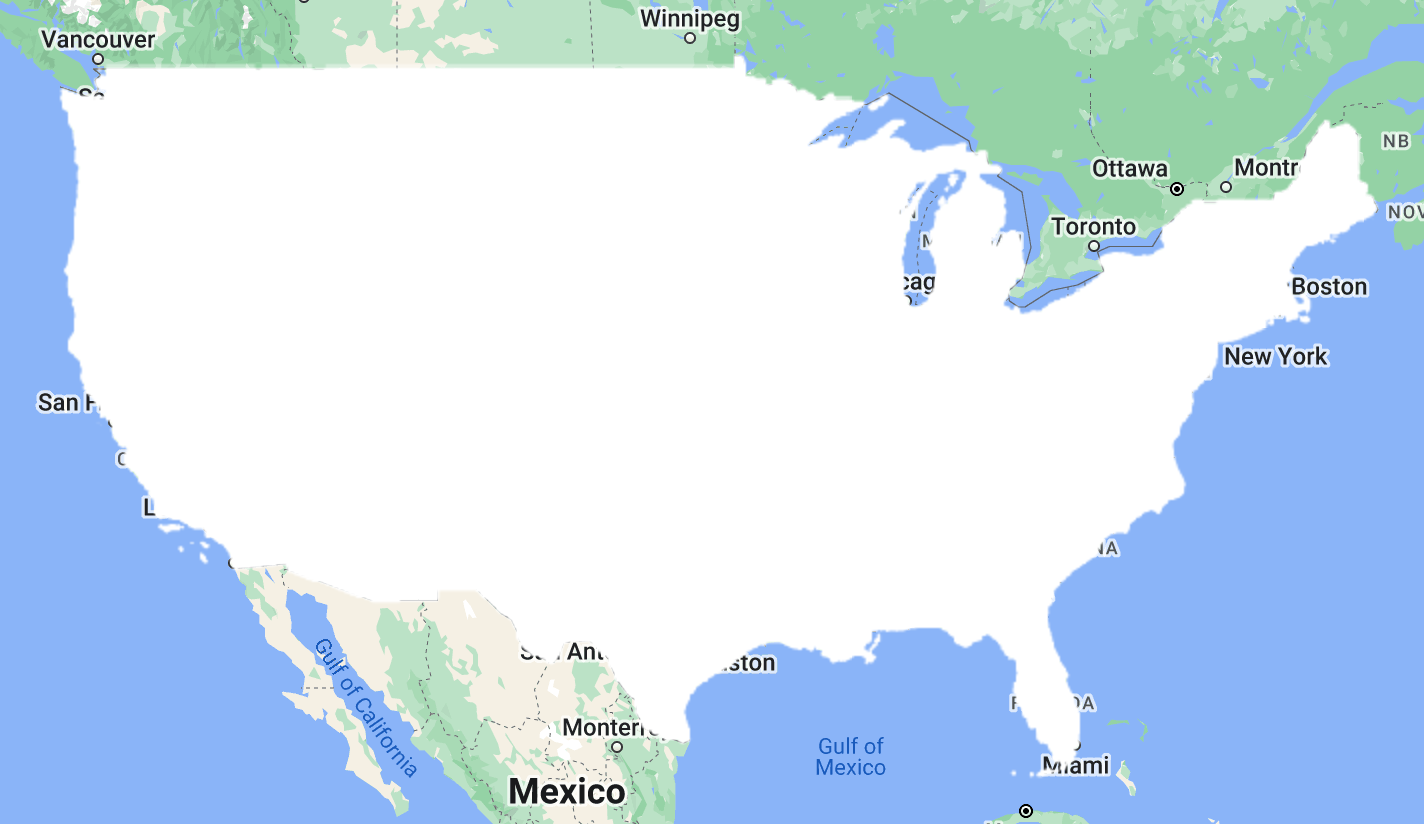
Our map looks like a white cutout. We can change properties of the layer using the Layers widget on the map. Hover over the Layers widget and hit the cog next to Layer 1. Select the option for
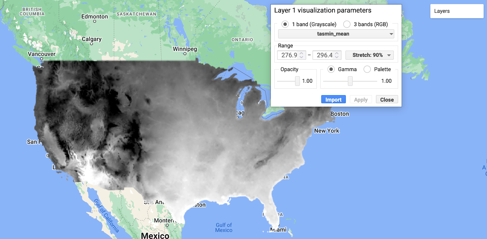
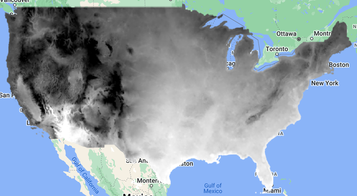
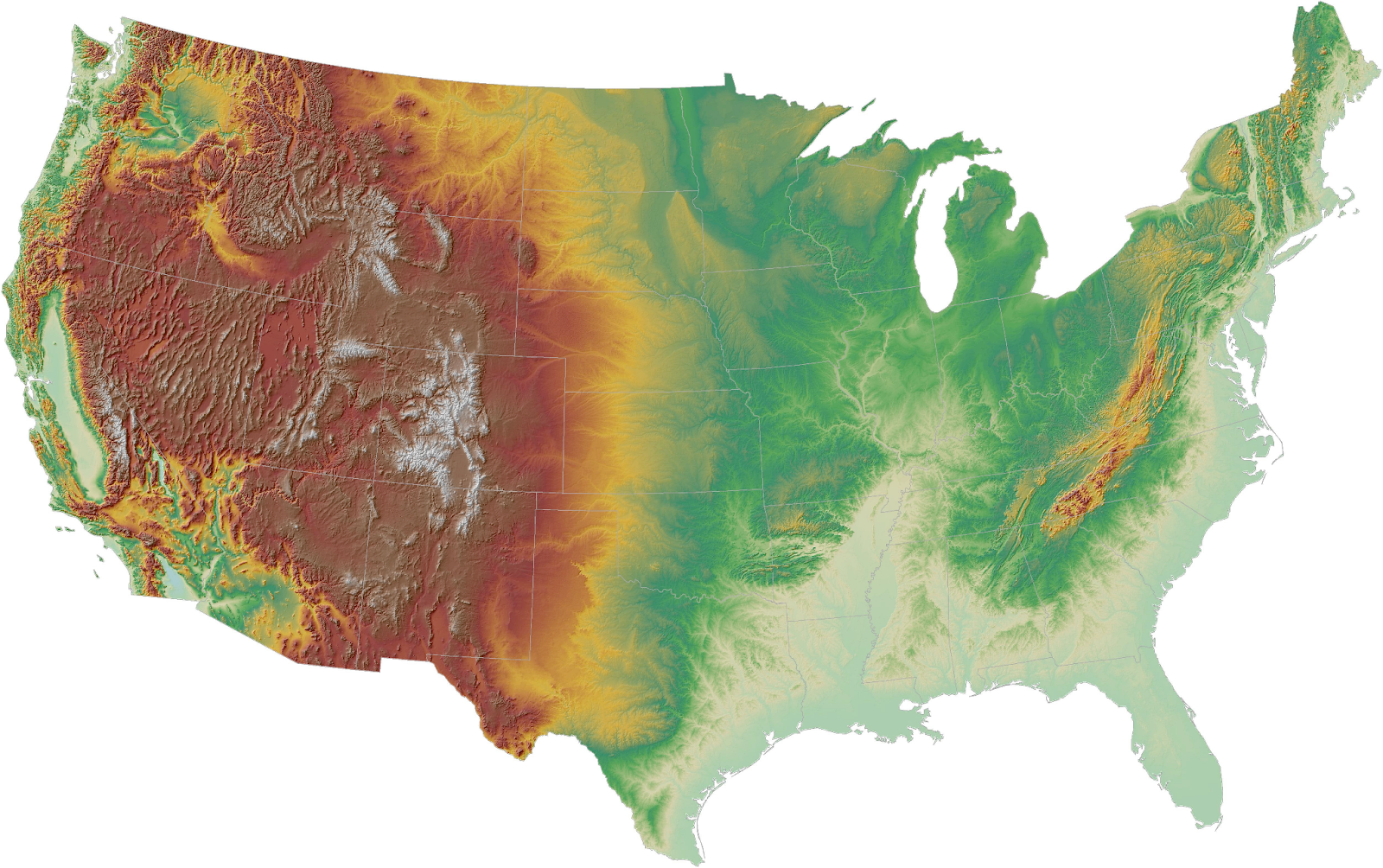
We now have a map showing mean minimum summertime temperatures for the period of 1950-1979. The dark spots are cooler temperatures and the whiter areas are warmer temperatures. The values are reported in Kelvin. Intuitively, areas with higher topography generally have colder temperatures such as over the Sierra Nevadas and the Rockies. Compare our map to a topographic map to see the temperature to elevation dependance.
Now, let’s create a raster for projected summertime temperature minimums using the RCP8.5 scenario (high emissions; business-as-usual).
Using the same set of methods with slightly modified inputs (we just changed which scenario we select and the date filter - that’s it!), we have generated an image (raster) of the projected summertime minimum temperatures under the RCP8.5 scenario.
Feel free to add this image to the map as another layer or not. We will now do simple raster math to compare these two images. We can subtract our historical temperatures from the projected temperatures to calculate how temperatures are projected to shift in the future.
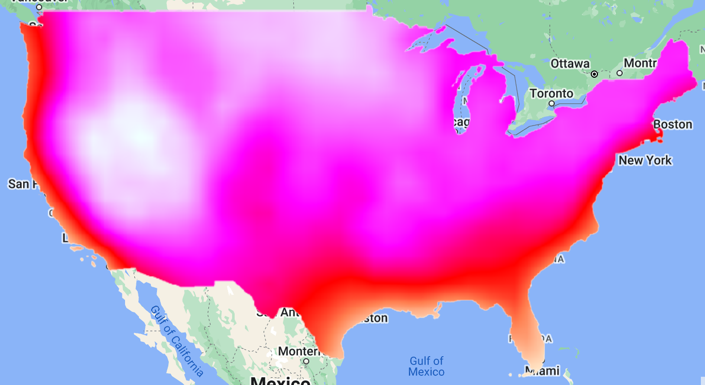
The minimum temperature change is 3.53 K (+6 deg F) and the maximum is 6.37 K (+11.47 deg F)! I found these values by adding the
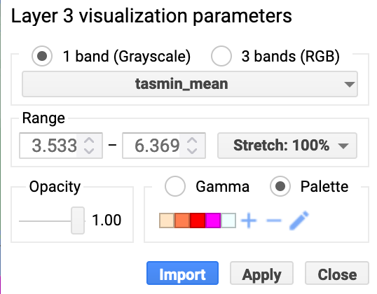
We now have a temperature change raster for the entire U.S. but let’s say you want to just clip a portion of the raster. We will learn two options:
>Use a state boundary feature (shape) already available in GEE
>Import our own shape file
Features - Shapes
Since GEE already has tons of geospatial data, a convenient first option is to explore the available datasets for your region of interest. If we want to clip the raster for just Illinois or any state boundary, you can imagine this might already be available in GEE. If we type into the search bar
Print this to the console to look at more details. We can now use the
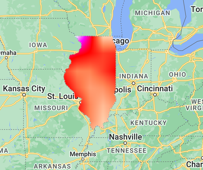
Importing data into GEE
If we find that GEE doesn’t have the shape or boundary we need, we are able to import our own shapes into GEE. As a reminder, shapes are called features in GEE. Let’s clip the Great Lakes subbasins using a shapefile from our labs. Grab the .zip of the shapefile from the USGS here: https://www.sciencebase.gov/catalog/item/530f8a0ee4b0e7e46bd300dd

Navigate to the
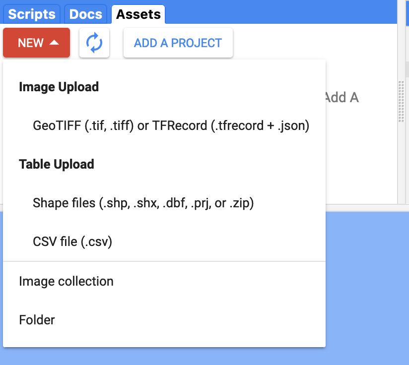
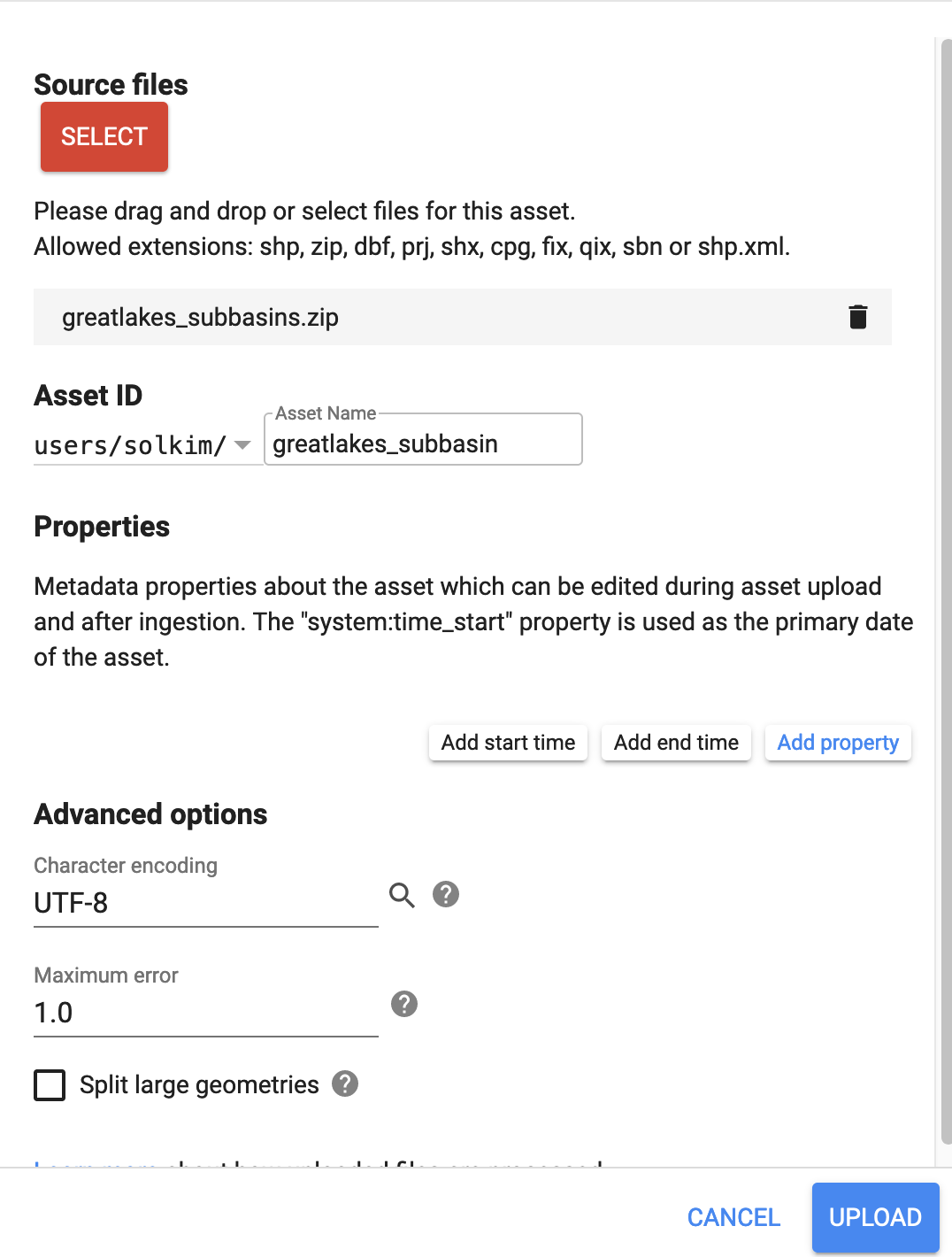
Once the Task has finished, if you navigate to your
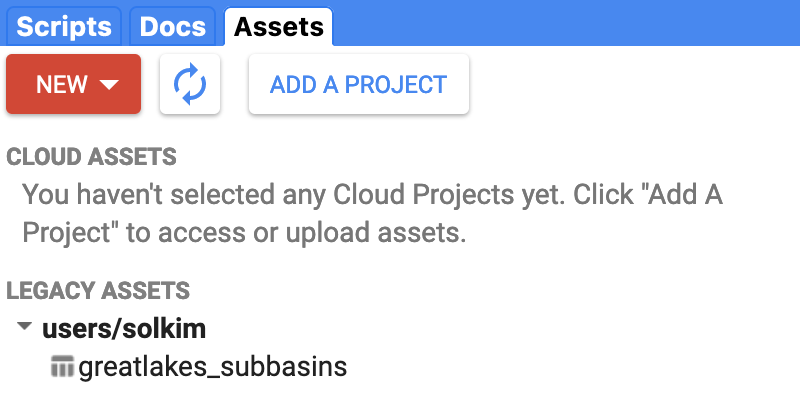
Click on the asset to pull up details of the asset and importantly, get the
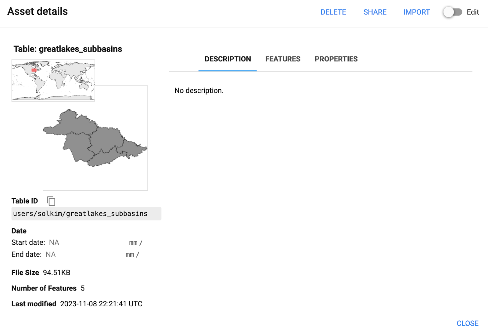
Add the following lines to the code editor but use your asset ID in place of mine (
If we examine the FeatureCollection, we should see 5 features corresponding to the 5 Great Lakes subbasins. For this exercise, let’s just clip the entire region and add it to the map.
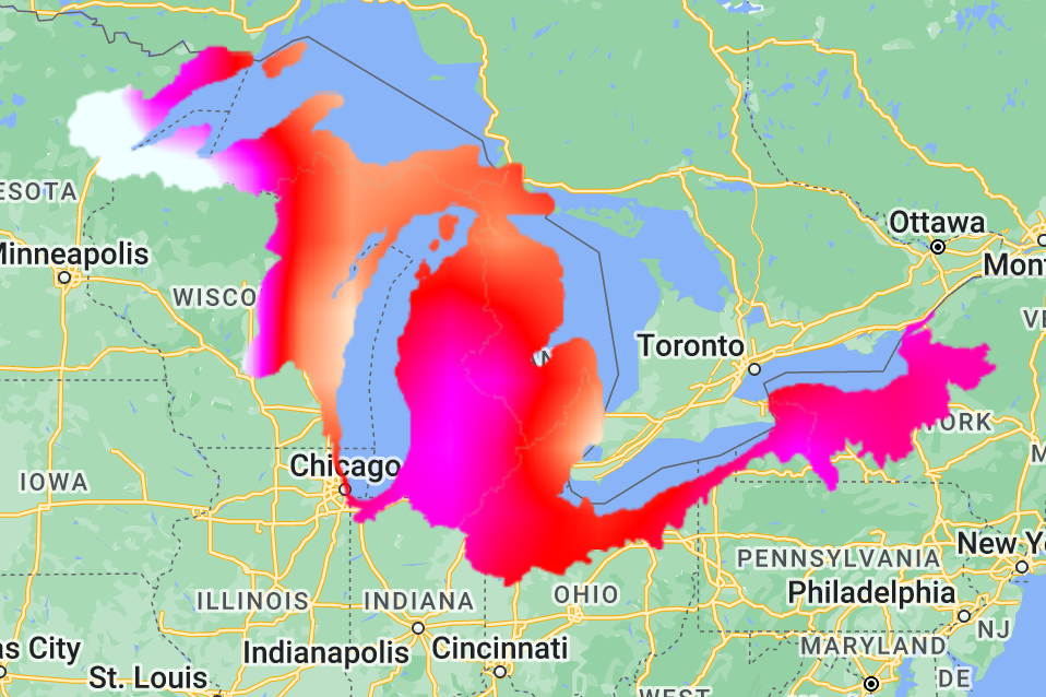
Exporting data out of GEE
We have processed and clipped rasters in GEE but let’s you want to work with this further in GIS. We can export images (rasters) and features (shapes) to our google drive. Export our Great Lakes temperature change raster with the following lines and hit run. In the Tasks tab on the right panel, you should see an option to run your unsubmitted export task. Hit
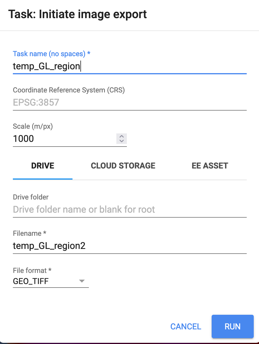
We can now bring in our clipped raster into QGIS for any further work.
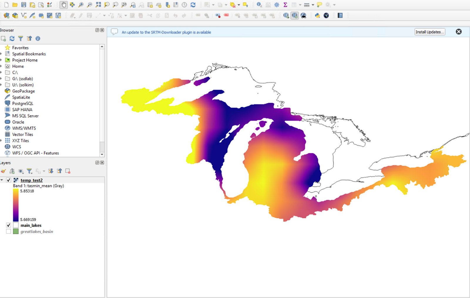
This tutorial is very brief and does not go into many details but the hope is that you learned what is capable with GEE and that with some simple tools, you can access the huge trove of datasets available and enable some pretty powerful analyses. Think about ways you can use GEE in your workflows for the project and beyond the class.
Clean Code
Below is a clean version of the tutorial. The imported data section is commented out as is the export to allow the whole block to run without issue for everyone.
A brief introduction to Google Earth Engine (GEE)
Premise and Objectives
This tutorial requires NO coding experience or familiarity with GEE. You MUST have an approved account to use GEE: https://earthengine.google.com/signup.
This tutorial will serve to act as a showcase of some capabilities that are possible with GEE. It is NOT meant to cover every detail of coding in GEE. We will cover a few basics of GEE using javascript (see note at the end about using python):
1. Overview
2. Datasets
3. Graphical User Interface (GUI)
4. Climate Projection - Rasters
5. Features - Shapes
6. Importing data into GEE
7. Exporting data out of GEE
8. Further resources
The workflow will specifically involve running a simple climate projection analysis using temperature over an imported shape area and exporting the results in a format we can use in GIS. If you ever get lost or run into errors, a clean working version of the code is posted at the end.
Overview
What is GEE? GEE is the most advanced cloud-based geospatial processing platform in the world. It combines a multi-petabyte catalog of satellite imagery and geospatial datasets with planetary-scale analysis capabilities and makes it available for scientists, researchers, and developers to detect changes, map trends, and quantify differences on the Earth's surface. https://earthengine.google.com/
• Unprecedented speed: On a top-of-the-line desktop computer, it can take days or weeks to compute an analysis over any large portion of the earth. Using our cloud-based computing power, we can reduce that by orders of magnitude.
• Ease of use and lower costs: An online platform that offers easy access to data, scientific algorithms, and computation power from any web browser can dramatically lower the cost and complexity for analysis of geospatial data.
Datasets
GEE has complete archives of Landsat 4,5,7, and 8 that have been processed by the United States Geological Survey (USGS), a wide variety of Moderate Resolution Imaging Spectro-Radiometer (MODIS) data products as global composites, and many other remotely-sensed and ancillary image data products. In recent years, GEE has been processing huge amounts of demographic data along with climate and weather data including outputs from climate models. All data are pre-processed, georeferenced, and ready for use. Users may also upload their own raster and vector data, which can be kept private or made publicly available. https://developers.google.com/earth-engine/datasets
In GEE, a single raster is an image while a collection of rasters is known as an image collection. Shapes are known as features and feature collections.
Graphical User Interface (GUI)
Access here: https://code.earthengine.google.com/
2. Access scripts, documentation on all GEE functions, and assets
3. Scripting window
4. Inspector, Console, Tasks
5. Map
Climate Projection - Rasters
We will begin by searching for climate model projections that are pre-processed in GEE. In the search bar, type
“Climate projection” and navigate to “NEX-DCP30: Ensemble Stats for NASA Earth Exchange Downscaled Climate Projections.”The data is monthly and spans from 1950-2099 with historical (1950-2005) and projected (2006-2099) runs. The projections are further split into three categories based on Representative Concentration Pathways or RCPs - RCP2.6, RCP4.5, and RCP8.5. These pathways represent different levels of greenhouse gas concentrations with the number next to “RCP” indicating the radiative forcing in W/m^2 (higher number = warmer climate). There are various variables we can work with such as precipitation or near surface temperature (see the
‘Bands’ tab). We will work with minimum near surface air temperature (tasmin_mean). Copy the Collection Snippet and close the dataset panel to return to the code editor.In the code editor, type:
var NEXDCP30 = ee.ImageCollection("NASA/NEX-DCP30_ENSEMBLE_STATS")
This line declares the variable
“NEXDCP30” and assigns it to the entire dataset we just inspected. Hit run (or Ctrl + Enter). Seemingly, nothing happens. To inspect our variable, we need to print it to the console. Add the following line and run:print(NEXDCP30)You should run into this error on your console (right panel). To preserve computation on GEE’s servers, GEE limits the query to 5000 elements. Instead of trying to grab the entire dataset, let’s just inspect the first image using the
first() method. var NEXDCP30 = ee.ImageCollection("NASA/NEX-DCP30_ENSEMBLE_STATS").first()
print(NEXDCP30)
If we go to the console tab, we should see our sample image with further information. Be sure to always do a check of your data in this way before trying any analysis so that you understand the organization of the data.
For a climate change analysis, we need a historical and a projected dataset to compare. We will use the first 3 decades from the historical runs (1950-1979) and last 3 decades from the projected runs (2070-2099) and examine how minimum surface temperatures during the summer have changed across the century. Climate analyses try to work with at least 3 decades of data to remove noise from natural year-to-year variability. Minimum temperatures can be thought of as nighttime temperatures while maximum temperatures can be thought of as the daytime temperatures. Under climate change, nighttime temperatures are increasing at a faster rate than daytime temperatures for most regions. During summer months, we rely on cool nighttime temperatures to recover from heat stress so being able to project the future trends is crucial with regards to human health. Let’s extract just what we need from the entire dataset as described above.
// Get the historical, minimum temperature, summertime mean

var climate_historical = ee.ImageCollection('NASA/NEX-DCP30_ENSEMBLE_STATS')

  .select('tasmin_mean') // Filter for only the minimum temperature variable/band

  .filter(ee.Filter.eq('scenario','historical')) // Filter for only historical runs

  .filter(ee.Filter.date('1950-01-01', '1979-12-31')) // Filter for the first 3 decades

  .filter(ee.Filter.calendarRange(6,8,'month')) // Filter only summer months (June-August, or months 6-8)

  .mean(); // Take the summertime mean of the entire 3 decades
The “//” indicates that the text that follows it is not meant to be evaluated but rather used as comments. Without getting into the weeds of each method, the code:
> first brings in the entire NEX-DCP30 ensemble image collection
> selects only the images in the collection that correspond to the band or variable we are interested in (
‘tasmin_mean’)> filters the images further for only the
‘historical' run> filters further for the first 3 decades
> filters further for the summer months
> finally take the mean of all the remaining images
If we
print(climate_historical), we should see it is now a single image (raster) with one band (tasmin_mean) which is what we want. To be clear, we now have a raster of mean summertime minimum surface temperature from the CMIP5 multi-model ensemble for 1950-1979. Let’s show this raster on our map by adding it as a layer.Map.setCenter(-100, 40, 4); // Set longitude and latitude with a zoom level
Map.addLayer(climate_historical,[],'historical'); // Add layer to map with a label
Our map looks like a white cutout. We can change properties of the layer using the Layers widget on the map. Hover over the Layers widget and hit the cog next to Layer 1. Select the option for
1 band (Grayscale) and set the range to “Stretch: 90%” or whichever you feel and hit Apply. *We will alter the map visuals using a code based method further along in the tutorial.We now have a map showing mean minimum summertime temperatures for the period of 1950-1979. The dark spots are cooler temperatures and the whiter areas are warmer temperatures. The values are reported in Kelvin. Intuitively, areas with higher topography generally have colder temperatures such as over the Sierra Nevadas and the Rockies. Compare our map to a topographic map to see the temperature to elevation dependance.
// Get the RCP8.5 projection, minimum temperature, summertime mean
var climate_projection = ee.ImageCollection('NASA/NEX-DCP30_ENSEMBLE_STATS')
.select('tasmin_mean') // Filter for only the minimum temperature variable/band
.filter(ee.Filter.eq('scenario','rcp85')) // Filter for only the RCP8.5 projection runs
.filter(ee.Filter.date('2070-01-01', '2099-12-31')) // Filter for only the last 3 decades
.filter(ee.Filter.calendarRange(6,8,'month')) // Filter only summer months (June-August, or months 6-8)
.mean(); // Take the summertime mean of the entire 3 decades
print('Projection:',climate_projection)
Using the same set of methods with slightly modified inputs (we just changed which scenario we select and the date filter - that’s it!), we have generated an image (raster) of the projected summertime minimum temperatures under the RCP8.5 scenario.
Feel free to add this image to the map as another layer or not. We will now do simple raster math to compare these two images. We can subtract our historical temperatures from the projected temperatures to calculate how temperatures are projected to shift in the future.
// Compare historical with projections using subtraction
var temp_change = climate_projection.subtract(climate_historical)
// Add temperature change to the map
Map.addLayer(temp_change,
{palette: 'ffe4c4,ff7f50,FF0000,FF00FF,f0ffff', // Color palette
min: 3.53, // Minimum value for color scale
max: 6.37, // Maximum value for colar scale
},'Temperature change'); // Name the layer
The minimum temperature change is 3.53 K (+6 deg F) and the maximum is 6.37 K (+11.47 deg F)! I found these values by adding the
temp_change layer to the map and going to the Layers widget, and setting the range to Stretch 100%. You may also notice that a color pallete has been added. Colors are added using their HEX values. You can choose colors with their HEX values here (https://g.co/kgs/7c7nGE) and add the colors programatically as I did (recommended) or you can do it through the Layer parameters by clicking the Layer widget (this option requires you to add the palette everytime you run the code). >Use a state boundary feature (shape) already available in GEE
>Import our own shape file
Features - Shapes
Since GEE already has tons of geospatial data, a convenient first option is to explore the available datasets for your region of interest. If we want to clip the raster for just Illinois or any state boundary, you can imagine this might already be available in GEE. If we type into the search bar
“US states”, under Tables (which is what features or shapes are listed under) we can see TIGER Census States 2016. This is a feature collection from the US Census Bureau contains all the state boundaries. Much like how we filtered an Image Collection, we can filter this feature collection to grab just the state we are interested in. Each feature has a “NAME” property and we can filter for “Illinois”. var illinois = ee.FeatureCollection('TIGER/2016/States').filter(ee.Filter.eq('NAME','Illinois'));Print this to the console to look at more details. We can now use the
clip() method to clip our temperature change raster with just the boundary of our Illinois feature and add it to the map.var temp_change_illinois = temp_change.clip(illinois)
Map.addLayer(temp_change_illinois,
{palette: 'ffe4c4,ff7f50,FF0000,FF00FF,f0ffff',
min: 5.72,
max: 5.97,
},'Temperature change IL'); Importing data into GEE
If we find that GEE doesn’t have the shape or boundary we need, we are able to import our own shapes into GEE. As a reminder, shapes are called features in GEE. Let’s clip the Great Lakes subbasins using a shapefile from our labs. Grab the .zip of the shapefile from the USGS here: https://www.sciencebase.gov/catalog/item/530f8a0ee4b0e7e46bd300dd
Navigate to the
Assets tab on the left panel and click New > Shape files. In the next panel, Select your downloaded .zip file and upload. This may take a few seconds or minutes. You can track the progress of the upload in the Tasks tab on the right panel. Once the Task has finished, if you navigate to your
Assets tab on the left side panel, we should see the “greatlakes_subbasins”.Click on the asset to pull up details of the asset and importantly, get the
Table ID which is the pathway to our uploaded shapefile. Copy the Table ID and close.Add the following lines to the code editor but use your asset ID in place of mine (
'users/solkim/greatlakes_subbasins')<- this will be different):// Grab the Great Lakes subbasin asset we uploaded
var greatlakes_subbasins = ee.FeatureCollection('users/solkim/greatlakes_subbasins') // Modify path for your asset!
print('Great Lakes Subbasins',greatlakes_subbasins)
If we examine the FeatureCollection, we should see 5 features corresponding to the 5 Great Lakes subbasins. For this exercise, let’s just clip the entire region and add it to the map.
var temp_change_greatlakes = temp_change.clip(greatlakes_subbasins)
Map.addLayer(temp_change_greatlakes,
{palette: 'ffe4c4,ff7f50,FF0000,FF00FF,f0ffff',
min: 5.61,
max: 5.93,
},'Temperature change GL'); Exporting data out of GEE
We have processed and clipped rasters in GEE but let’s you want to work with this further in GIS. We can export images (rasters) and features (shapes) to our google drive. Export our Great Lakes temperature change raster with the following lines and hit run. In the Tasks tab on the right panel, you should see an option to run your unsubmitted export task. Hit
RUN to bring up a panel with further options (format should be GEO_TIFF) and hit Run again. This process will take a minute or two and you should find your GEOTIFF in your google drive!// Export the GL region to our google drive
Export.image.toDrive({
image: temp_change, // The image to export
description: 'temp_GL_region', // Short description
region: greatlakes_subbasins, // The region to export (clip)
maxPixels: 1e9 // Max pixels for our image (prevents errors)
})We can now bring in our clipped raster into QGIS for any further work.
This tutorial is very brief and does not go into many details but the hope is that you learned what is capable with GEE and that with some simple tools, you can access the huge trove of datasets available and enable some pretty powerful analyses. Think about ways you can use GEE in your workflows for the project and beyond the class.
Clean Code
Below is a clean version of the tutorial. The imported data section is commented out as is the export to allow the whole block to run without issue for everyone.
// Tutorial + Demo for ICSM au23
// Climate Change - Projected summertime temperatures
// A + G + S
// Import sample of NASA NEX-DCP30 Ensemble Stats Image Collection
var sample = ee.ImageCollection("NASA/NEX-DCP30_ENSEMBLE_STATS").first(); // Grab just the first image to inspect properties
print('My sample image:', sample)
// Get the historical, minimum temperature, summertime mean
var climate_historical = ee.ImageCollection('NASA/NEX-DCP30_ENSEMBLE_STATS')
.select('tasmin_mean') // Filter for only the minimum temperature variable/band
.filter(ee.Filter.eq('scenario','historical')) // Filter for only historical runs
.filter(ee.Filter.date('1950-01-01', '1979-12-31')) // Filter for the first 3 decades
.filter(ee.Filter.calendarRange(6,8,'month')) // Filter only summer months (June-August, or months 6-8)
.mean(); // Take the summertime mean of the entire 3 decades
print('Historical:',climate_historical)
// Get the RCP8.5 projection, minimum temperature, summertime mean
var climate_projection = ee.ImageCollection('NASA/NEX-DCP30_ENSEMBLE_STATS')
.select('tasmin_mean') // Filter for only the minimum temperature variable/band
.filter(ee.Filter.eq('scenario','rcp85')) // Filter for only the RCP8.5 projection runs
.filter(ee.Filter.date('2070-01-01', '2099-12-31')) // Filter for only the last 3 decades
.filter(ee.Filter.calendarRange(6,8,'month')) // Filter only summer months (June-August, or months 6-8)
.mean(); // Take the summertime mean of the entire 3 decades
print('Projection:',climate_projection)
// Add historical and projection means to the map
Map.setCenter(-100, 40, 4); // Set longitude and latitude with a zoom level

Map.addLayer(climate_historical,[],'historical'); // Add layer to map with a label
Map.addLayer(climate_projection,[],'projection');
// Compare historical with projections using subtraction

var temp_change = climate_projection.subtract(climate_historical)


// Add temperature change to the map

Map.addLayer(temp_change,

{palette: 'ffe4c4,ff7f50,FF0000,FF00FF,f0ffff', // Color palette

min: 3.53,  // Minimum value for color scale

max: 6.37,  // Maximum value for colar scale

},'Temperature change'); // Name the layer
// Grab the Illinois state boundary and add it to the map
var illinois = ee.FeatureCollection('TIGER/2016/States').filter(ee.Filter.eq('NAME','Illinois'));
Map.addLayer(illinois,[],'Illinois')
// // Grab the Great Lakes subbasin asset we uploaded
// var greatlakes_subbasins = ee.FeatureCollection('users/solkim/greatlakes_subbasins') // Modify path for your asset!
// print('Great Lakes Subbasins',greatlakes_subbasins)
// Clip the temperature with the Illinois boundary and the Great Lakes boundary
var temp_change_illinois = temp_change.clip(illinois)
// var temp_change_greatlakes = temp_change.clip(greatlakes_subbasins)
// Add these to the map with their own scaling
Map.addLayer(temp_change_illinois,
{palette: 'ffe4c4,ff7f50,FF0000,FF00FF,f0ffff',
min: 5.72,
max: 5.97,
},'Temperature change IL');
// Map.addLayer(temp_change_greatlakes,
// {palette: 'ffe4c4,ff7f50,FF0000,FF00FF,f0ffff',
// min: 5.61,
// max: 5.93,
// },'Temperature change GL');
// // Export the GL region to our google drive
// Export.image.toDrive({
// image: temp_change, // The image to export
// description: 'temp_GL_region', // Short description
// region: greatlakes_subbasins, // The region to export (clip)
// maxPixels: 1e9 // Max pixels for our image (prevents errors)
// })
- Tutorials and documentation: https://developers.google.com/earth-engine/guides/getstarted
-
Earth Engine Fundamentals and Applications *this is a great resource to learn: https://www.eefabook.org/go-to-the-book.html
-
Python: https://developers.google.com/earth-engine/guides/python_install
-
Datasets: https://developers.google.com/earth-engine/datasets
-
JRC Global Surface Water Animations: https://showcase.earthengine.app/view/jrc-global-surface-water-animation
-
TROPOMI pollution: https://showcase.earthengine.app/view/tropomi-explorer
-
Turbidity app: https://code.earthengine.google.com/4fac188d66c71e0972f843c12508347b
-
Mississippi River Basin Floodplain Landuse change:
- https://gee-community-catalog.org/projects/floodplain_lc/?h=mississippi